Use Cases

With the pykCSD toolbox you can estimate 1D, 2D and 3D potentials and CSD based on your input data. Here are the basic examples for each of the reconstructions.

Sample 1D reconstruction

You can estimate potentials measured with electrodes placed along a line:

from pykCSD.pykCSD import KCSD
import numpy as np

#the most inner list corresponds to a position of one electrode
elec_pos = np.array([[-0.5], [0], [1], [1.5], [3.5], [4.1], [5.0], [7.0], [8.0]])

#the most inner list corresponds to a time recording made with one electrode
pots = np.array([[-0.1], [0.3], [-0.4], [0.2], [0.8], [0.5], [0.2], [0.5], [0.6]])

#you can define model parameters as a dictionary
params = {
        'xmin': -3.0,
        'xmax': 12.0,
        'source_type': 'gauss',
        'n_sources': 30
}

k = KCSD(elec_pos, pots, params)

k.estimate_pots()
k.estimate_csd()

k.plot_all()

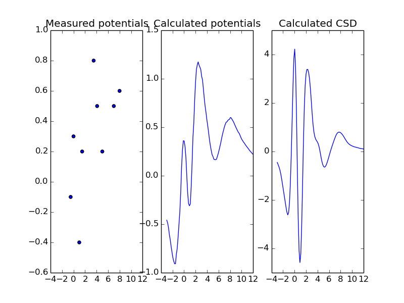
The sample reconstruction in 1D

Cross validation

Having your kCSD solver set up, you can use cross validation to regularize your results:

from pykCSD import cross_validation as cv
from sklearn.cross_validation import LeaveOneOut

index_generator = LeaveOneOut(len(elec_pos), indices=True)
lambdas = np.array([10000./x**2 for x in xrange(1, 50)])

k.solver.lambd = cv.choose_lambda(lambdas, pots, k.solver.k_pot, elec_pos, index_generator)

print k.solver.lambd

k.estimate_pots()
k.estimate_csd()

k.plot_all()

>> 4.16493127863

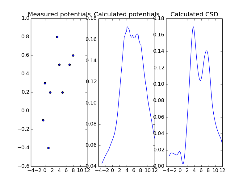
The same reconstruction regularized with cross validation

Sample 2D reconstruction

You can estimate potentials and CSD measured with planar electrodes:

from pykCSD.pykCSD import KCSD
import numpy as np

elec_pos = np.array([[-0.2, -0.2],[0, 0], [0, 1], [1, 0], [1,1], [0.5, 0.5], [1.2, 1.2]])
pots = np.array([[-1], [-1], [-1], [0], [0], [1], [-1.5]])
params = {'gdX': 0.05, 'gdY': 0.05, 'xmin': -2.0, 'xmax': 2.0, 'ymin': -2.0, 'ymax': 2.0}

k = KCSD(elec_pos, pots, params)

k.estimate_pots()
k.estimate_csd()

k.plot_all()

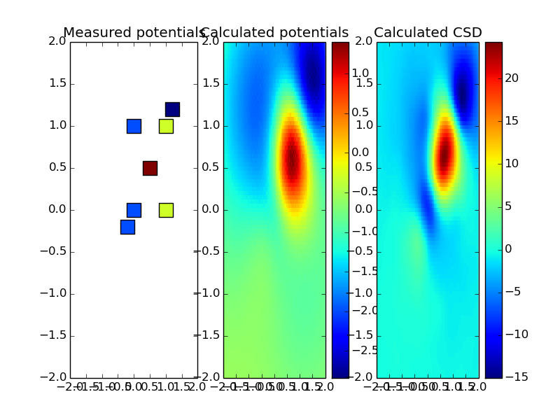
The sample reconstruction in 2D

Sample 3D reconstruction

You can also recostruct CSD and LFP using measurements taken by spatial electrodes:

from pykCSD.pykCSD import KCSD
import numpy as np

elec_pos = np.array([(0, 0, 0), (0, 0, 1), (0, 1, 0), (1, 0, 0),
                        (0, 1, 1), (1, 1, 0), (1, 0, 1), (1, 1, 1),
                        (0.5, 0.5, 0.5)])
pots = np.array([[-0.5], [0], [-0.5], [0], [0], [0.2], [0], [0], [1]])
params = {
        'gdX': 0.05,
        'gdY': 0.05,
        'gdZ': 0.05,
        'n_sources': 64,
}
k = KCSD(elec_pos, pots, params)

k.estimate_pots()
k.estimate_csd()

k.plot_all()

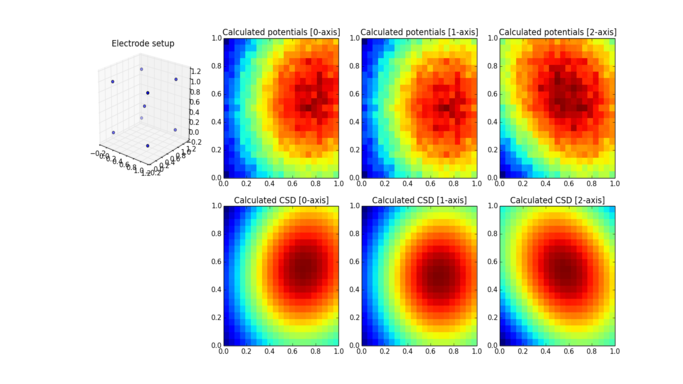
The sample reconstruction in 3D

Such a dataset can be also visualized using mayavi:

from mayavi import mlab

csd = k.solver.estimated_csd[:,:,:,0]
#setting up a proper gui backend
%gui wx
mlab.pipeline.image_plane_widget(mlab.pipeline.scalar_field(csd),
                        plane_orientation='x_axes',
                        slice_index=10,
                        )
mlab.pipeline.image_plane_widget(mlab.pipeline.scalar_field(csd),
                        plane_orientation='y_axes',
                        slice_index=10,
                        )
mlab.outline()

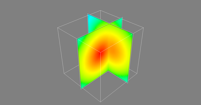
The same reconstruction visualized with mayavi